Proud supporter of:
		Helping Children With Autism

Gravity Bowl Motion

The following describes the mathematics and control issues that are important to coordinating the motion of the GravityBowl highly maneuverable electric vehicle.

Figure 1: Wheel arrangement and definition of motion parameters.

Equations of Motion

Figure 1 shows the configuration of the three wheels and the coordinate frame used here. Given time-dependent position of the center of the vehicle and time dependent orientation, the following equations describe the positions of the three wheel centers 0, 1 and 2 at their locations of 0, 120 and -120 degrees around the vehicle:

(1)

where r is the radius of the vehicle at the wheel attachment points. These equations can be differentiated to give the velocity equations which describe the instantaneous ground velocity at each wheel center:

(2)

Note that these velocities depend on the forward velocity of the vehicle, the rotational speed and the instantaneous orientation, .

Steering Angle and Speed

It is useful to compute the steering angle , which is the orientation of the velocity vector at each wheel center relative to the orientation of the vehicle. This angle is given by:

(3)

The speed of motion of each wheel is equal to the magnitude of the velocity vector:

(4)

Steering Vectors

Instead of using the steering angle and speed it can be more useful to work out the velocity vector of each wheel in the coordinate frame of the vehicle, rather than in the frame of the ground plain. To do this we simply convert to a vector (polar to rectangular conversion). Rather than using trig for this, we can get the same result more conveniently by rotating the three velocity vectors from (2) through an angle using a rotation matrix, so the wheel velocity vector in GravityBowl coordinates, , is now given by

(5)

This leads to

(6)

These are the main equations that we need to work with.

By way of example, when the overall velocity vector is zero, but rotational speed is non-zero, the three steering angles are given by and corresponding to wheel velocities of , and . These are independent of. In this case, the vehicle is simply turning about its center and the steering angles reflect the tangential velocity. In this case, wheel speed is equal to as would be expected.

The meaning of bears a little explanation: This angle is the time integral of the angular speed which means that it linearly increases for constant positive. Of course if is varying then it could increase or decrease. The steering control system needs to integrate over time to maintain the correct wheel velocities. The constant of integration (value of at time zero) gives the heading of the vehicle because it sets the direction of initial motion.

Analysis of Motion

There are two ways of thinking about the motion of the vehicle, depending on whether you are looking at it from the point of view of the ground plain or of someone sitting on the vehicle. If the vehicle rotates and translates then an observer outside will see the vehicle move along a fixed direction and rotate about its moving center. Equations (2) describe this scenario. Alternatively, from the perspective of a passenger there is no rotation. Instead, the forward motion of the vehicle looks like a motion vector that spins around as the vehicle moves. This is described by the set of equations (6).

Figure 2: Three modes of motion. Note that the circle here indicates the length of the vectors produced by rotation; it is not the GravityBowl outline.

Let’s use equations (2) to visualize how the motion changes for each wheel over time. In this case there is one translational velocity vector and to this gets added to three different vectors that each depend on the rotation speed. This is shown in the left diagram of Figure 2 where vectors 0, 1, and 2 are components for the respective wheels. These three vectors have length and rotate around as changes as indicated by the circle in the diagram. When is small compared with then the resultant vectors all have about the same orientation and vary around the direction of as indicated by the left diagram. The three steering angles swing around with but all have a similar direction.

The next important situation arises when equals as indicated by the center diagram. Here, the resultant vectors become zero and reverse direction as passes through critical angles. On the right hand diagram, the vehicle is spinning faster than it is moving. In this case, the velocity vectors remain approximately tangential to the vehicle perimeter.

Alternatively we can look at what happens from the viewpoint of the vehicle in which case we use equations (6). Figure 3 indicates this situation. There are three tangential velocity components of length which remain fixed relative to the vehicle. To these are added a velocity component which is the same for each wheel but rotates around with angular speed , i.e. backwards. The steering angle is given by the resultant vector and the wheel speed by its length. It is clear from this diagram that the wheels will stop and reverse once per cycle when .

Figure 3: Wheel velocities in relative to the vehicle. The center circle is the outline of the GravityBowl.

We can use a computer simulation to help us understand what happens in a realistic case. Here we consider two scenarios of motion: accelerating linear velocity and accelerating rotation.

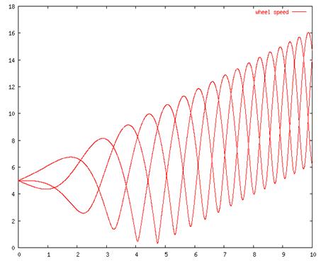
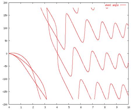
Consider the case when the vehicle is initially at rest but is spinning about its center. From this position we accelerate the vehicle along the x-axis with constant acceleration. Figure 4 shows graphs of steering angle and wheel speed for this situation. The vehicle passes through the three modes of Figure 2 from to . From these graphs it can be seen that steering angle can change very rapidly near the condition that (at around t=4) and can switch instantaneously through 180°.

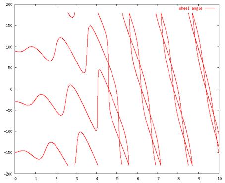
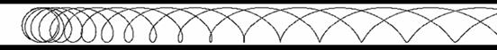
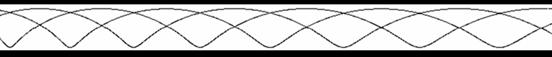
Figure 5 shows what happens when the vehicle is initially moving along the x-axis but slowly begins to rotate. Similar mode transitions occur as in Figure 4 but in the opposite direction. The ground tracks of the wheels for the two different types of acceleration described here are plotted in Figure 6.

Figure 7 shows the three modes as a graph. Independent control of and will always produce this behavior. It can only be avoided by a different parameterization that appropriately links and to avoid the large swings in steering angle. An example of such a parameterization would be tricycle motion as described later.

Figure 4: Graph of wheel speed (top) and angle (bottom) for constant velocity but accelerating rotation.

Figure 5: Graph of wheel speed (top) and angle (bottom) for constant rotation but accelerating horizontal motion.

Figure 6: Motion tracks made by the three wheels. Top: Constant velocity, accelerating rotation. Bottom: Constant rotation, accelerating horizontal motion.

Figure 7: Graph showing regions of different types of motion.

Wheel Skid and Velocity Error

The steering angles and wheel speeds form a six dimensional space which can be parameterized by the velocity vectors, however the region of this space for which there is no wheel slipping is three dimensional (because we have two dimensions of ground velocity and one of orientation.) An example of a wheel slip configuration is one for which all wheels point inwards and such configurations are undesirable. If we naively command the wheels to arbitrary speeds and angles we will obtain some motion but a lot of skidding. It is useful to compute the nearest legitimate steering parameters from an arbitrary set of steering commands. It is also useful to work out the size of the error between actual steering angles and wheel speeds and the desired theoretical non-slipping angles and speeds. The reason that this might be useful is that in practice we cannot control the wheels perfectly and their behavior will always lag behind any control signal that we send to them. Even if we command the wheels to the perfect non-slipping time-varying configurations they will not reach these desired trajectories. We would like to know how much unwanted slippage this error produces because slippage will be related to undesirable frictional forces and wheel side loads.

We can compute the ground velocity and rotational speed that would result from an arbitrary set of wheel velocities (in the vehicle reference frame). The ground velocity is given by the average of the wheel velocities, rotated through angle:

(7)

Likewise we can work out an “average” value for because each wheel vector contributes a rotational component tangential to the vehicle edge and this can be computed via a dot product. The final formula works out to be:

(8)

Let’s use vector notation and let. Using the formulae above we can now compute the nearest “correct” set of wheel velocities W from a given set U which may include slippage. We can do this by multiplying by a matrix A, so that. We can then find the error vector which directly represents the amount of slippage produced by U. The error vector will be given by which when evaluated, turns out to be

(9)

We can use this error measure to indicate the extent of slippage over time by evaluating the magnitude of the vector E. We will use this result in the future when we need to check the performance of the servo systems.

We can check the above result by putting the equations for W from (6) into this formula in place of U. In this case E turns out to be zero indicating that any valid steering vectors fall into the null space of this matrix.

Tricycle Motion

One simple method of steering is to keep two “back” wheels at a steering angle parallel to the direction of travel and steer with a “front” wheel. The configuration for this is shown in Figure 8.

Figure 8: Geometry of tricycle configuration.

Let us use to denote the speed of wheel 0. In this case the velocity vector for wheel 0 is given by

(10a)

The angular speed of motion around the turning center Z is given by . This allows us to work out the speeds of the two remaining wheels which are and . Using trig we can eliminate d and R to obtain:

(10b)

These equations show that when turning left, wheel 1 moves slower than while wheel 2 moves faster than which is as expected if no slipping occurs. If we put these equations for W into the error equation in place of U then we find E is zero which helps to verify the result.

We can now use equations (7) and (8) to calculate the motion of the vehicle in terms of its ground velocity and the rotation about its center point:

(11)

and

. (12)

As one might expect, the tricycle turns in a circle of radius R and vectorrotates at a rate that depends on the value of which itself depends on the steering angle.